In this article we will discuss the concept of probability. We will review the main interpretations of probability, among with their incompatibilities.
Then, we will explain how the axiomatic approach resolves such inconsistencies.
Definitions of Probability
Intuitively, probability can be seen as the likelihood of an event occurring. In probability theory, many different formlizations of this key concept have been done.
Classical probability
The first and so-called classical approach to probability have been formalized by the notorious mathematician Pierre-Simon Laplace in his work Théorie analytique des probabilités:
The probability of an event is the ratio of the number of cases favorable to it, to the number of all cases possible when nothing leads us to expect that any one of these cases should occur more than any other, which renders them, for us, equally possible.
We can formalize the definition above even further. Let $A$ be an event. Then:
This definition is simple, intuitive and very easily appliable to a vast number of scenarios. Hence we can immediately see its drawbacks: each event must have the exact same probability.
As an example, let’s consider the roll of a dice with 6 possible outcomes. Let us examine the event $A_i$ such that $A_i$ occurs if the outcome of a dice roll is $i$. Then:
Nevertheless, we must notice that if the dice is weighted, then it is not anymore true that all the events $A_i$ have the same likelihood. The definition of classical probability does not support such scenario.
Frequentist probability
The frequentism can be thought as an approach to probability that is more close to statistics. It can be defined as the relative frequency of an event in an infinite number of trials.
We can try to give a more formal definition of the frequentist probability. Let $A$ be an event, $N_n(A)$ be the number of occurrences of $A$ in $n$ trials. Then:
We can immediately notice the empirical nature of frequentism. While this approach can potentially lead to easier analyses for complex phoenomena, its major drawback is that it may not be appliable to non-repeatable events.
Bayesian probability
Bayesianism is an approach to probability partly based on belief. An introductory definition of Bayesian probability is given by ScienceDirect:
Bayesian probability is defined as a probability that is relative to evidence, used to analyze statistical inferences by incorporating prior information and rational degrees of belief. It is characterized by its application in decision-making and hypothesis testing, generating updated probabilities at the conclusion of statistical tests.
The key idea of Bayesianism is that, given an uncertain hypothesis which can be either true or false, we give a prior probability partly based on belief (therefore potentially biased). Then, we can use evidence (i.e. newly acquired relevant data) to update it to a posterior probability.
Bayes theorem
The Bayes theorem is crucial in probability theory. Formally, it allows to define the joint probability of two events $H$ and $D$ in terms of conditioned probability:
Deriving the last two terms of the equation above, we can obtain the mostly usual formulation of the Bayes theorem:
Now, let $H$ be our hypothesis and $D$ be the evidence data. We can derive the Bayes theorem to formulate a so-called posterior distribution:
where each $h$ is a possible outcome of the $H$ random variable.
Geometric probability
Geometric probability is a powerful approach to deal with probability when an event is represented as a continuous random variable (i.e. its spectrum is a continuous interval).
An example of how geometric probability works is given in a beautiful article by brilliant.org. Let’s say we are waiting for the bus. Let $X \in [0,60]$ be a random variable representing the time of arrival of the bus. If the bus arrives between $0$ and $30$ (i.e. $X \in [0,30]$), we miss the bus, otherwise we catch it.
It is clear that in this scenario the definitions of probability given earlier cannot be applied. For example, we cannot even define a number of possible outcomes for a continuous interval. However, we can model the problem in a geometric fashion. Let’s define $X$ geometrically (credits brilliant.org):
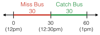
We can easily understand that in this case $\Pr(X) = \frac{1}{2}$, as we can compare the probabilities of arrival times collectively as lengths of segments.
The axiomatic approach
The axiomatic approach in probability was introduced by Andrey Kolmogorov in 1933, in its work Foundations of the theory of probability. They provide an unambiguous and strict foundation for probability theory.
To quote a great quality article from the Berkeley University:
The Kolmogorov axioms are technically useful in providing an agreed notion of what is a completely specified probability model within which questions have unambiguous answers. This eliminates cases like Bertrand’s paradox which is simply an ambiguously defined model. But they encourage both a false sense of security (that the act of formulating a model within the mathematical framework somehow guarantees it is a valid representation of the real world phenomenon) and a narrowness of vision (that aspects of the real world that cannot be formulated within the framework are somehow “not probability”).
Kolmogorov axioms
In his works, Kolmogorov defined three axioms to formalize the notion of probability. First, the following context is requried:
- let $\Omega$ be the sample space, i.e. the set of all possible outcomes
- let $F$ be the space of events; $F$ must be a $\sigma$-algegra of $\Omega$
- let $\Pr(A)$ be the probability measure, assigning a probability value to each event $A \in F$
Using the context above as a base, we can give the actual Kolmogorov axioms:
- The probability of an event is always non-negative, i.e.:
$$ \Pr(A) \ge 0 \quad \forall\ A \in F $$
- The probability that at least one outcome $\omega \in \Omega$ will occur is
equal to $1$:
$$ \Pr(\Omega) = 1 $$
It follows that $0 \le \Pr(A) \le 1 \quad \forall\ A \in F$.
- For every $E_i$ such that all $E_i$ are mutually exclusive
(i.e. $\Pr(E_j \cup E_k) = 0 \ \forall\ j,k$) it holds:
$$ \Pr\left( \ \bigcup_{i=1}^\infty E_i \right) = \sum_{i=1}^\infty P(E_i) $$
Derived property
Subadditivity property
Let $A, B \in F$ be two events. First, notice that the following holds:
This statement allows us to use the third axiom, as $A$ and $B \setminus A$ are always disjoint. By the third axiom follows:
As $B \subseteq B \setminus A$, it follows that:
Inclusion-exclusion principle
Let $A, B \in F$ be two events. Simply by the properties of sets, the following decomposition holds:
Then, by the third Kolmogorov axiom:
In the previous section, we have already seen that the following holds:
Then: