In this article we will perform a simulation of $n$ events occurring over a time span $[0,T]$ at a rate $\lambda$. The time span will be a continuous interval, so we will not be able to apply the principles relative to the classical approach towards probability.
We will also perform a further theoretical analysis of the stochastic process, identifying the theoretical distributions involved and discussing the relative properties.
Simulation
Metodology and resources
As in the previous article, we will use the rust programing language to implement the code to perform the simulations and plot the relative data. As already explained, such approach will allow to perform simulations in a blazing-fast, safe and efficient way.
The rand crate has been used to simulate single
events. It is the de-facto standard forrandom number simulation in rust.
The plotters crate has been used to generate
charts out of simulation data.
Code infrastructure
First, let’s implement a simulator to abstract the infrastructure according to the context parameters such as $n$ and $\lambda$:
use rand::{distr::Bernoulli, prelude::*};

#[derive(Debug, Clone)]
pub struct Simulator {
    /// Full time period
    pub t: f32,

    /// Time definition (i.e. number of trials)
    pub n: u32,

    /// Success rate
    pub lambda: f32,
}

impl Simulator {
    /// Instance a new simulator
    pub fn new(t: f32, n: u32, lambda: f32) -> Self {
        Self { t, n, lambda }
    }

    /// Generate a simulation
    pub fn run(&self) -> Simulation {
        let p = (self.lambda as f64) / (self.n as f64);

        let bernoulli = Bernoulli::new(p).unwrap();
        let rng = rand::rng();

        let mut data: Vec<i32> = Vec::with_capacity(self.n as usize);
        let mut sum: i32 = 0;

        for success in bernoulli.sample_iter(rng).take(self.n as usize) {
            sum += if success { 1 } else { 0 };
            data.push(sum);
        }

        Simulation(data)
    }
}
In one of the previous articles we used the
rand::Rng::random_bool method to directly simulate a Bernoulli trial. This
time, we will use the rand::distr::Bernoulli facility, which may be faster
for repeated trials with the same distribution according to the official
rand
documentation.
Also, the Bernoulli::sample_iter method can be used to iterate over n
random trials in a very elegant way.
We can also model a generated simulation as a type, so we can tailor it to our
specific needs. Rust’s trait system (in particular the
Deref and
IntoIterator)
will allow us to conveniently treat our custom type as an array of trials if
needed.
use std::ops::Deref;

pub struct Simulation(Vec<i32>);

impl Deref for Simulation {
    type Target = Vec<i32>;

    fn deref(&self) -> &Self::Target {
        &self.0
    }
}

impl<'a> IntoIterator for &'a Simulation {
    type Item = &'a i32;
    type IntoIter = std::slice::Iter<'a, i32>;

    fn into_iter(self) -> Self::IntoIter {
        self.0.iter()
    }
}

impl Simulation {
    pub fn final_value(&self) -> i32 {
        self.0.last().copied().unwrap_or(0)
    }
}
Plotting charts
As in the already mentioned previous article, we will use the plotters and
clap crates to craft a handy and convenient CLI utility. The relative code is
given immediately below.
use clap::Parser;
use homework_07::*;
use plotters::prelude::*;

#[derive(Parser)]
#[command(name = "poisson", about = "Poisson simulator and plotter")]
struct Cli {
    /// Full time period
    #[arg(short, default_value = "1")]
    pub t: f32,

    /// Time definition (i.e. number of trials)
    #[arg(short, default_value = "1000")]
    pub n: u32,

    /// Success rate
    #[arg(short, long)]
    pub lambda: f32,

    /// Width of the graph in pixels
    #[arg(short = 'W', long, default_value = "1920")]
    pub width: u32,

    /// Height of the graph in pixels
    #[arg(short = 'H', long, default_value = "1080")]
    pub height: u32,

    /// Output file
    #[arg(short, long)]
    pub output: String,
}

fn main() {
    let args = Cli::parse();
    let sim = Simulator::new(args.t, args.n, args.lambda).run();

    let root = BitMapBackend::new(&args.output, (args.width, args.height)).into_drawing_area();
    root.fill(&WHITE).unwrap();

    let y_max: i32 = sim.iter().max().copied().unwrap_or(args.n as i32);
    let caption = format!(
        "Poisson simulation with t={}, n={}, lambda={} - Last value: {}",
        args.t,
        args.n,
        args.lambda,
        sim.final_value(),
    );

    let mut chart = ChartBuilder::on(&root)
        .caption(caption, ("sans-serif", 24))
        .margin(20)
        .x_label_area_size(40)
        .y_label_area_size(40)
        .build_cartesian_2d(0.0..args.t as f64, 0..y_max)
        .unwrap();

    chart
        .configure_mesh()
        .x_desc("Time")
        .y_desc("Value")
        .draw()
        .unwrap();

    let data: Vec<(f64, i32)> = sim
        .iter()
        .enumerate()
        .map(|(i, v)| (i as f64 * args.t as f64 / args.n as f64, *v))
        .collect();
    chart.draw_series(LineSeries::new(data, RED)).unwrap();

    root.present().unwrap();
}
We can invoke the CLI tool directly with cargo:
$ cargo run --bin plotter -- --help
Poisson simulator and plotter

Usage: plotter [OPTIONS] --lambda <LAMBDA> --output <OUTPUT>

Options:
  -t <T>                 Full time period [default: 1]
  -n <N>                 Time definition (i.e. number of trials) [default: 1000]
  -l, --lambda <LAMBDA>  Success rate
  -W, --width <WIDTH>    Width of the graph in pixels [default: 1920]
  -H, --height <HEIGHT>  Height of the graph in pixels [default: 1080]
  -o, --output <OUTPUT>  Output file
  -h, --help             Print help
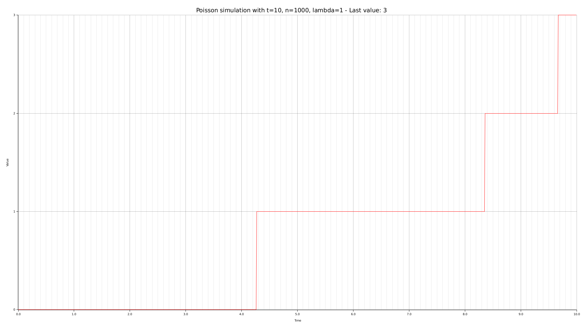
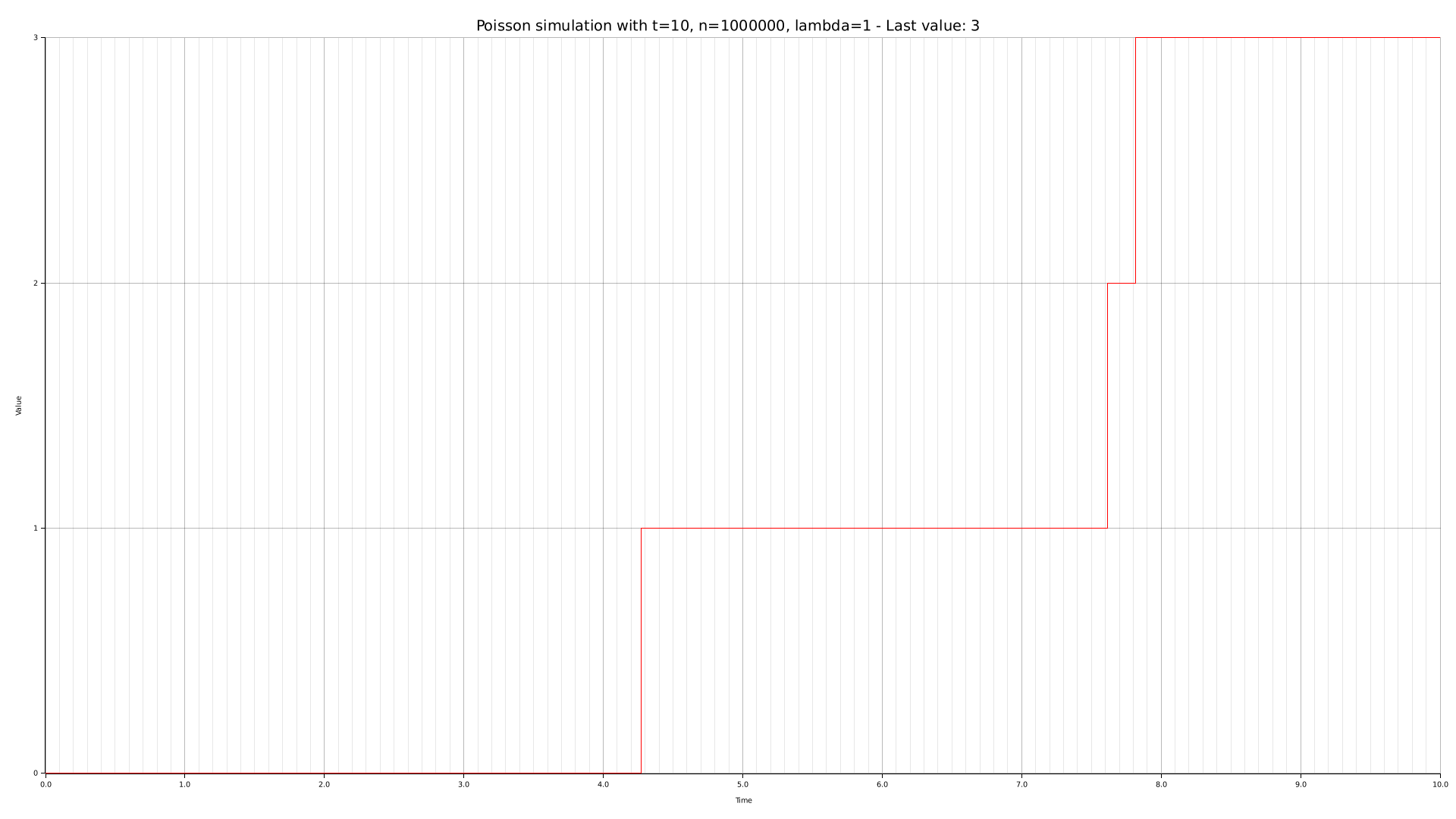
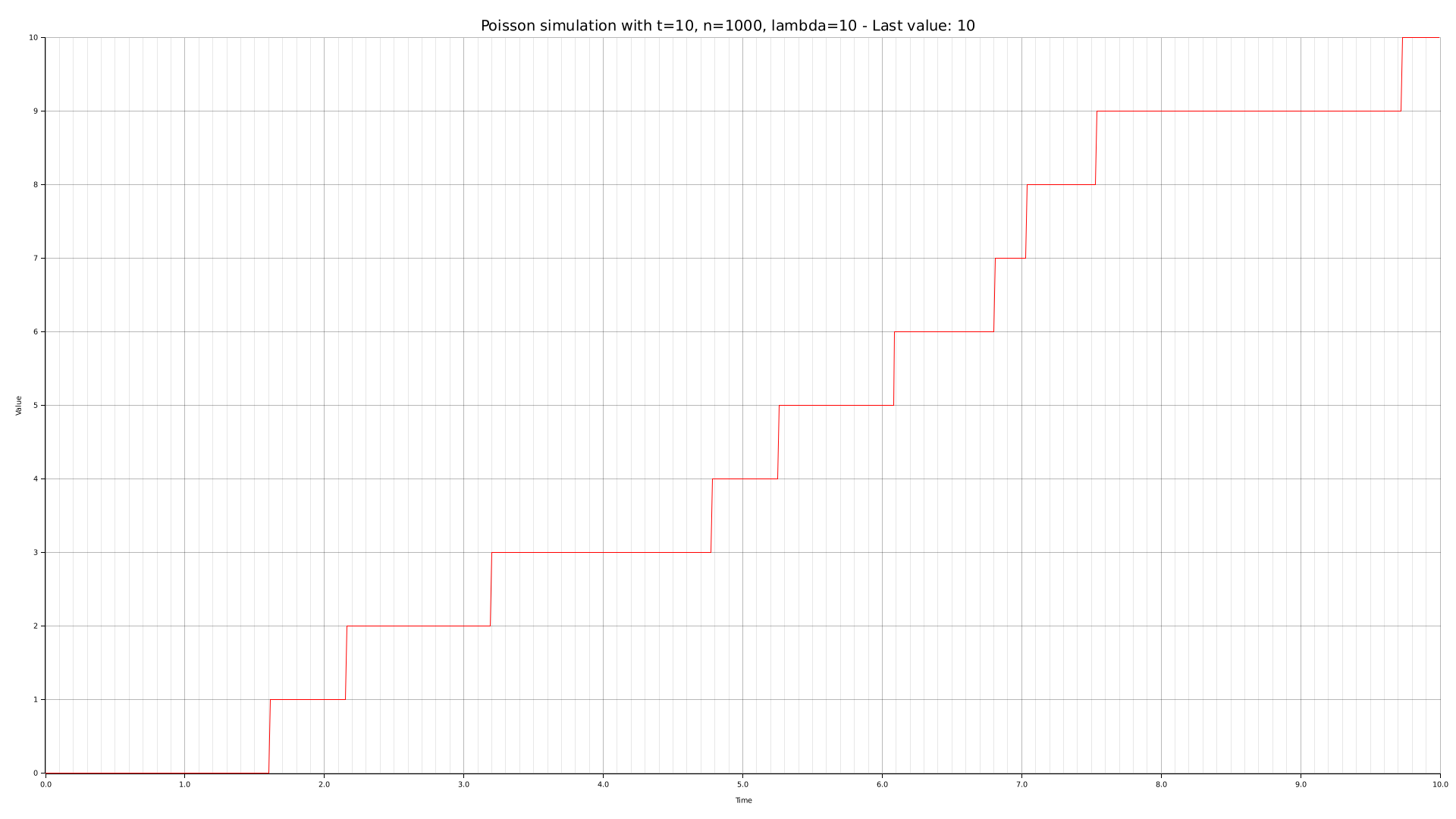
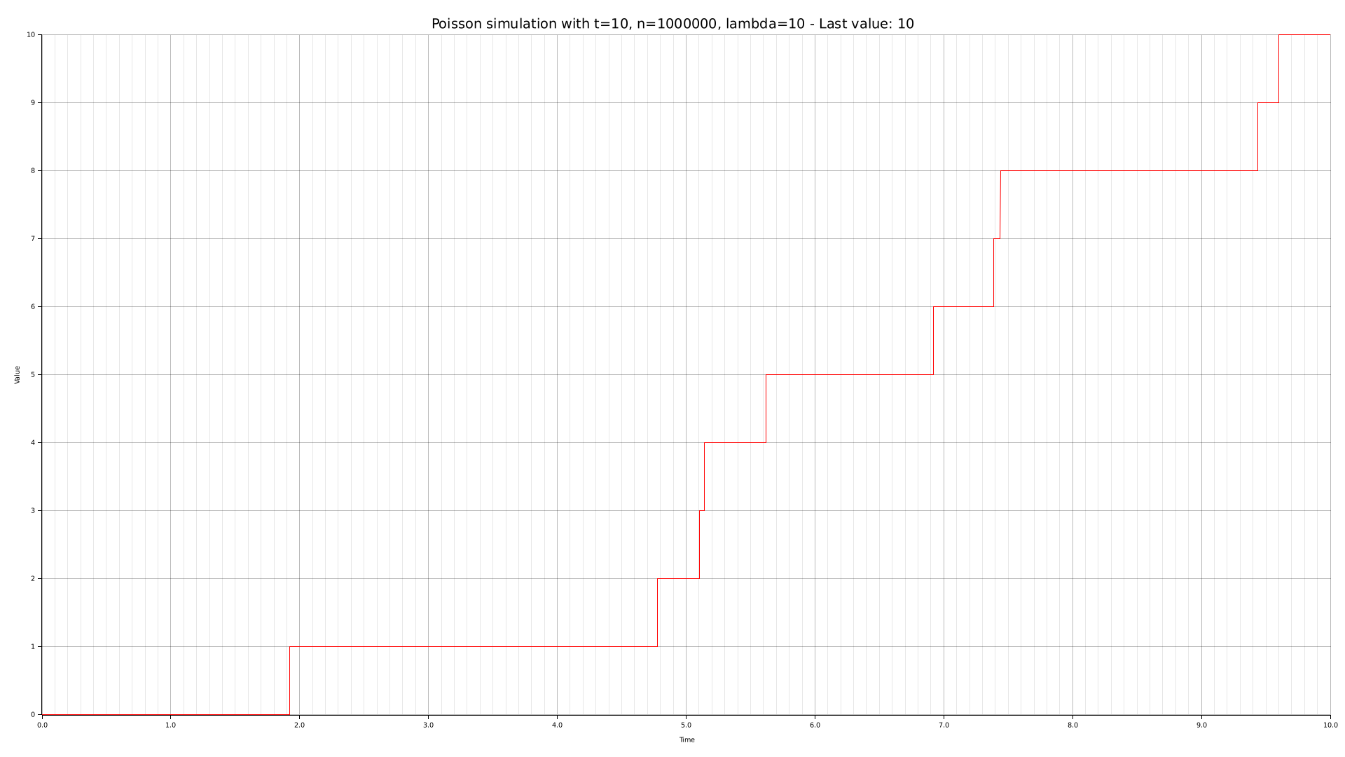
Running the simulation
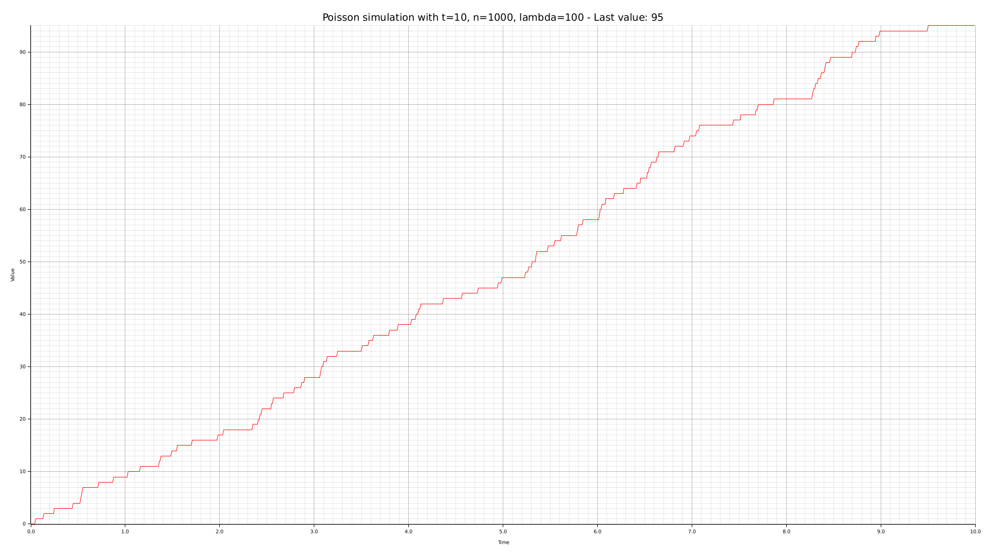
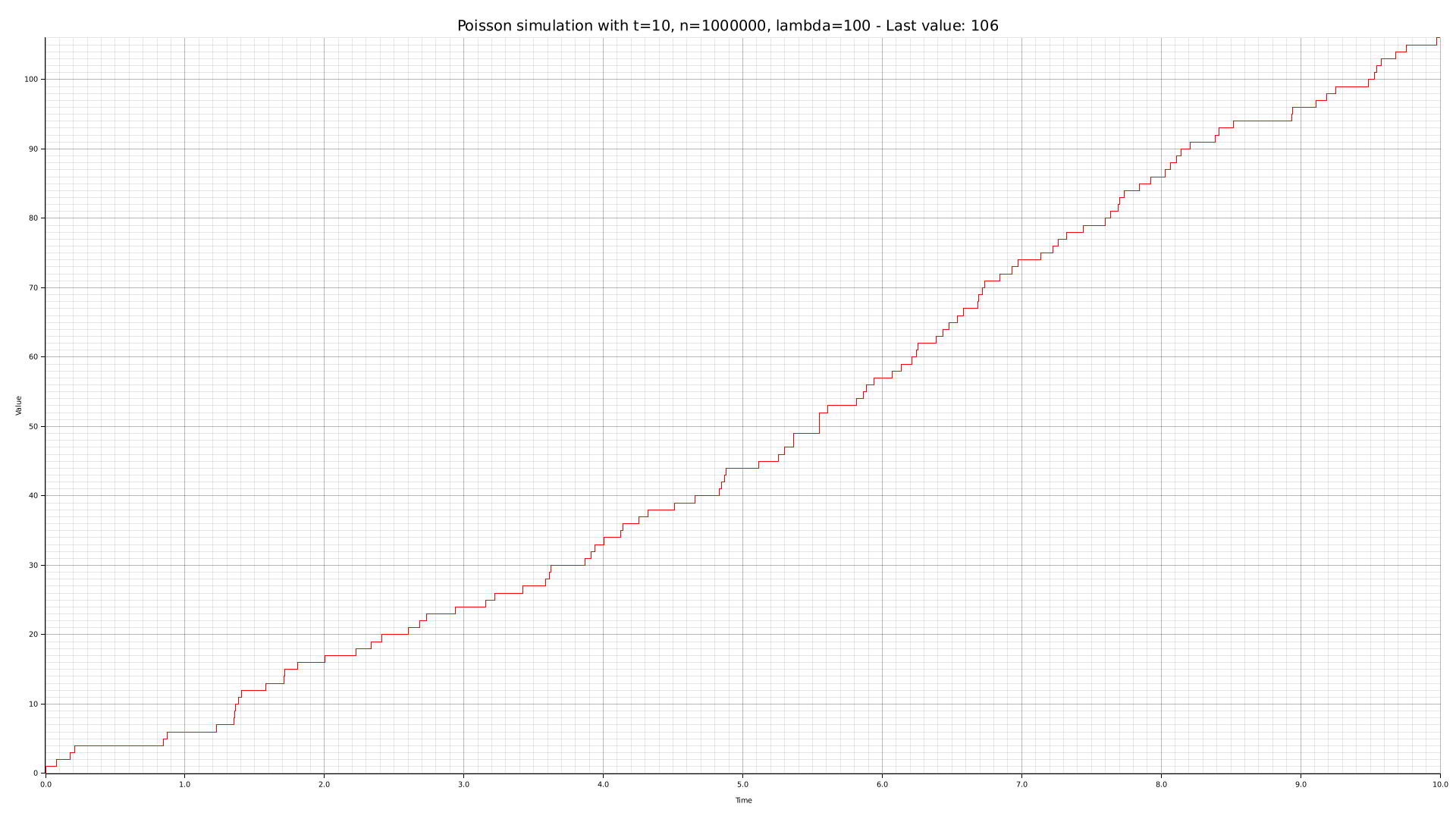
To obtain an empirical basis for our posterior theoretical analysis, we are going to generate some charts with the CLI tool we crafted. Such graphs are given below, along with their relative parameters.
Theoretical analysis
Stochastic process
The performed simulation approximates a notorious distribution known as the Poisson distribution. Such distribution models the expectation of $lambda$ successes over a continuous time span $[0,T]$.
In order to emulate a Poisson distribution, the time span $[0,T]$ is divided into $n$ samples. At each sample, there is a $\frac{\lambda}{n}$ probability of success. Naturally, the higher $n$ is, the closer to a Poisson distribution the simulation is.
Let $X \sim \text{Pois}(\lambda)$. Given an arbitrary value $k$, the probability mass function gives us the probability of $X = k$:
Binomial convergence
Strictly speaking, the simulation we did actually perform a Binomial stochastic process with $p = \frac{\lambda}{n}$. Moreover, we also said that it emulates a Poisson distribution. We can deduce that a Binomial distribution theoretically converges to a Poisson when $n \to \infty$:
On the $\lambda$ parameter
We already said the $\lambda$ parameter represents the expected number of successes over a time span $[0,T]$.
We know that for a Binomial distribution the expected value is:
Moreover, we know that a Bernoulli converges to a Poisson distribution when $n \to \infty$. So we can conclude: