In this article we will simulate the cybersecurity assesment of a production server using random walks.

Theoretical background

Bernoulli distribution

In a previous article we mentioned the Bernoulli random variable. We will now explore the topic of random variables more in depth.

The Bernoulli random variable is a discrete variable that can be defined as follows:

$$ X \sim \text{Bernoulli} (p) = \begin{cases} 1 & \text{with probability } p \\ 0 & \text{with probability } q = 1 - p \end{cases} $$

The Bernoulli variable and distribution can be used to model binary events (i.e. events that can either success or fail, e.g. a coin toss) with arbitrary probability.

Binomial distribution

The Binomial distribution is used to model repeated Bernoulli trials. Let $Y_i \sim \text{Bernoulli}(p) \ \forall \ i \in [1..n]$. We can define the Binomial random variable as follows:

$$ X \sim B(p) = \sum_{i=0}^n Y_i $$

Rademacher distribution

The Rademacher random variable is defined as follows:

$$ X \sim \text{Rad}(p) = \begin{cases} 1 & \text{with probability } p \\ -1 & \text{with probability } q = 1 - p \end{cases} $$

Unsurprisingly, the Rademacher distribution can be (and usually is) expressed in terms of the Bernoulli distribution. Let $Y \sim \text{Bernoulli}(p)$. Then:

$$ X \sim \text{Rad}(p) = 2 Y - 1 $$

We can prove this relation very straightforwardly:

$$ \begin{split} Y = 1 & \implies X = 2 Y - 1 = 2 \cdot 1 - 1 = 1 \\ Y = 0 & \implies X = 2 Y - 1 = 2 \cdot 0 - 1 = -1 \end{split} $$

Random walks

Quoting the definition of the Merriam-Webster dictionary, a random walk is:

a process (such as Brownian motion or genetic drift) consisting of a sequence of steps (such as movements or changes in gene frequency) each of whose characteristics (such as magnitude and direction) is determined by chance

We can model a random walk in the following way. Let $X_i \sim \text{Bernoulli}(p) \ \forall \ i \in [1,n]$. Imagine that, while moving forward, we can go either left or right. At each Bernoulli trial $X_i$, if $X_i = 0$ we move left, otherwise we move right.

A random walk can be obtained even more easily using the Rademacher distribution. If we repeat $n$ Rademacher trials and plot the result in a line chart, the line itself represents the walk. Further, we will see this more in depth.

Server score simulation

We will consider an exposed server which is upgraded every week for $n$ weeks. Each week the server is attacked by hackers. The perpetrated cyberattacks can either be successful or fail. If the server is violated, the score is decremented by $1$; if not, the score is incremented by $1$.

Formal problem definition

We will define a formal problem out of the above specification. Let:

$$ X_i \sim \text{Rad}(p) = \text{"the server is violated"} = \begin{cases} 1 & \text{if the server is violated} \\ -1 & \text{otherwise} \end{cases} $$

Let $s_i$ be the score of the server at the $i$-th week. Then:

$$ s_i = \begin{cases} 0 & \text{if } i = 0 \\ s_{i-1} - X_i & \text{if } i \ne 0 \end{cases} $$

Notice how $s_i$ is defined in terms of a concurrent relation.

Of course, the Rademacher distribution could be easily replaced with a Bernoulli, hence using the first one it is even more trivial to define $s_i$.

Implementing the simulation

In all the previous articles, all the proposed implementation were given in JavaScript. This time, we will make a step further and implement our simulation in rust. Rust is a compiled, strongly-typed, blazing-fast, memory-safe language that has some incredible features.

Introduction to rust projects

First, let’s initialize a rust library project:

cargo init --lib homeworks/homework-07

The cargo utility is the official all-in-one tool to manage packages and projects in rust.

Rust library projects are very convenient to work with. The embedded test framework is quite powerful and convenent, and they even support the creation of multiple standalone binaries.

Let’s see what cargo created for us:

$ cd homeworks/homework-07
$ ls
Cargo.toml src

The Cargo.toml file is used for the project configuration. It contains stuff like metadata and dependencies. The src directory contains the actual source code.

Generating random walks

First, let’s model a simulator to generate random walks with arbitrary parameters:

#[derive(Debug, Clone)]
pub struct Simulator {
    /// Number of weeks
    pub n: u32,

    /// Number of attackers
    pub m: u32,

    /// Probability of violating the server
    pub p: f32,
}

We will also model the outcome of a simulation with a dedicated type:

pub struct RandomWalk(Vec<i32>);

impl Deref for RandomWalk {
    type Target = Vec<i32>;

    fn deref(&self) -> &Self::Target {
        &self.0
    }
}

impl<'a> IntoIterator for &'a RandomWalk {
    type Item = &'a i32;
    type IntoIter = std::slice::Iter<'a, i32>;

    fn into_iter(self) -> Self::IntoIter {
        self.0.iter()
    }
}

impl RandomWalk {
    pub fn final_value(&self) -> i32 {
        self.0.last().copied().unwrap_or(0)
    }
}

Supplying implementation for the Deref and IntoIterator traits allows us to use any instance of RandomWalk as a vector of numbers while using all the advantages of having a dedicated type for it.

Implementing the actual algorithm to generate random walks is quite straightforward:

impl Simulator {
    pub fn new(n: u32, m: u32, p: f32) -> Self {
        Self { n, m, p }
    }

    /// Generate a random walk
    pub fn random_walk(&self) -> RandomWalk {
        let mut rng = rand::rng();
        let mut walk: Vec<i32> = Vec::with_capacity(self.n as usize);
        let mut sum: i32 = 0;

        for _ in 0..self.n {
            sum += self.random_step(&mut rng) as i32;
            walk.push(sum);
        }

        RandomWalk(walk)
    }

    /// Generate a random step
    fn random_step(&self, rng: &mut ThreadRng) -> i8 {
        let violated = (0..self.m)
            .map(|_| rng.random_bool(self.p as f64))
            .any(|v| v);
        if violated { -1 } else { 1 }
    }
}

Notice that the way we implemented the algorithms above allows us to reuse a single Simulator instance to generate multiple random walks.

Plotting random walks

To plot the random walks, we will use the awesome clap and plotters libraries to implement a highly flexible CLI utility. First, let’s define the allowed parameters of the CLI utility. The clap library allows us to do it in a very clean and idiomatic way using derive macros:

#[derive(Parser)]
#[command(name = "walk", about = "Random walk generator and plotter")]
struct Cli {
    /// Number of weeks
    #[arg(short)]
    pub n: u32,

    /// Number of attackers
    #[arg(short, default_value = "1")]
    pub m: u32,

    /// Probability of violating the server.
    /// If not specified, it will be computed such that the probability of violating the server at
    /// least once is 0.5
    #[arg(short)]
    pub p: Option<f32>,

    /// Number of different trajectories.
    /// A simulation will be performed for each trajectory
    #[arg(short, long, default_value = "1")]
    pub trajectories: u32,

    /// Width of the graph in pixels
    #[arg(short = 'W', long, default_value = "1920")]
    pub width: u32,

    /// Height of the graph in pixels
    #[arg(short = 'H', long, default_value = "1080")]
    pub height: u32,

    /// Output file
    #[arg(short, long)]
    pub output: String,
}

We can examine the result of what’s above by running:

$ cargo run --bin plotter -- --help  // Somewhat like ./plotter --help, but cargo builds and runs the utility for us

Random walk generator and plotter

Usage: plotter [OPTIONS] -n <N> --output <OUTPUT>

Options:
  -n <N>                             Number of weeks
  -m <M>                             Number of attackers [default: 1]
  -p <P>                             Probability of violating the server. If not specified, it will be computed such that the probability of violating the server at least once is 0.5
  -t, --trajectories <TRAJECTORIES>  Number of different trajectories. A simulation will be performed for each trajectory [default: 1]
  -W, --width <WIDTH>                Width of the graph in pixels [default: 1920]
  -H, --height <HEIGHT>              Height of the graph in pixels [default: 1080]
  -o, --output <OUTPUT>              Output file
  -h, --help                         Print help

Notice that we can plot multiple random walks in the same chart.

With the plotters library we can actually present our simulation in a line chart:

fn main() {
    let args = Cli::parse();
    let p = args.p.unwrap_or_else(|| compute_fair_p(args.m, 0.5));

    let sim = Simulator::new(args.n, args.m, p);
    let walks: Vec<RandomWalk> = (0..args.trajectories).map(|_| sim.random_walk()).collect();

    let root = BitMapBackend::new(&args.output, (args.width, args.height)).into_drawing_area();
    root.fill(&WHITE).unwrap();

    let (y_min, y_max) = y_bounds(&walks, args.n as i32);
    let x_max = args.n as i32;

    let caption = if args.trajectories == 1 {
        let final_value = walks.get(0).unwrap().final_value();
        format!(
            "Random walk with n={}, m={}, p={:.3} - Last value: {}",
            args.n, args.m, p, final_value,
        )
    } else {
        format!("Random walk with n={}, m={}, p={:.3}", args.n, args.m, p)
    };

    let mut chart = ChartBuilder::on(&root)
        .caption(caption, ("sans-serif", 24))
        .margin(20)
        .x_label_area_size(40)
        .y_label_area_size(40)
        .build_cartesian_2d(0..x_max, y_min..y_max)
        .unwrap();

    chart
        .configure_mesh()
        .x_desc("Time (weeks)")
        .y_desc("Server score")
        .draw()
        .unwrap();

    for w in walks {
        let w: Vec<(i32, i32)> = w
            .as_slice()
            .iter()
            .enumerate()
            .map(|(i, v)| (i as i32, *v))
            .collect();
        chart
            .draw_series(LineSeries::new(w, &random_color()))
            .unwrap();
    }

    root.present().unwrap();
}

fn compute_fair_p(m: u32, target: f32) -> f32 {
    1.0 - (1.0 - target).powf(1.0 / (m as f32))
}

fn y_bounds(walks: &Vec<RandomWalk>, n: i32) -> (i32, i32) {
    let y_min = walks.iter().flatten().min().copied().unwrap_or(-n);
    let y_max = walks.iter().flatten().max().copied().unwrap_or(n);
    (y_min, y_max)
}

fn random_color() -> RGBColor {
    let mut rng = rand::rng();
    RGBColor(
        rng.random_range(0..=255),
        rng.random_range(0..=255),
        rng.random_range(0..=255),
    )
}

Running the simulation

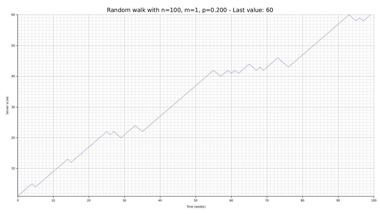
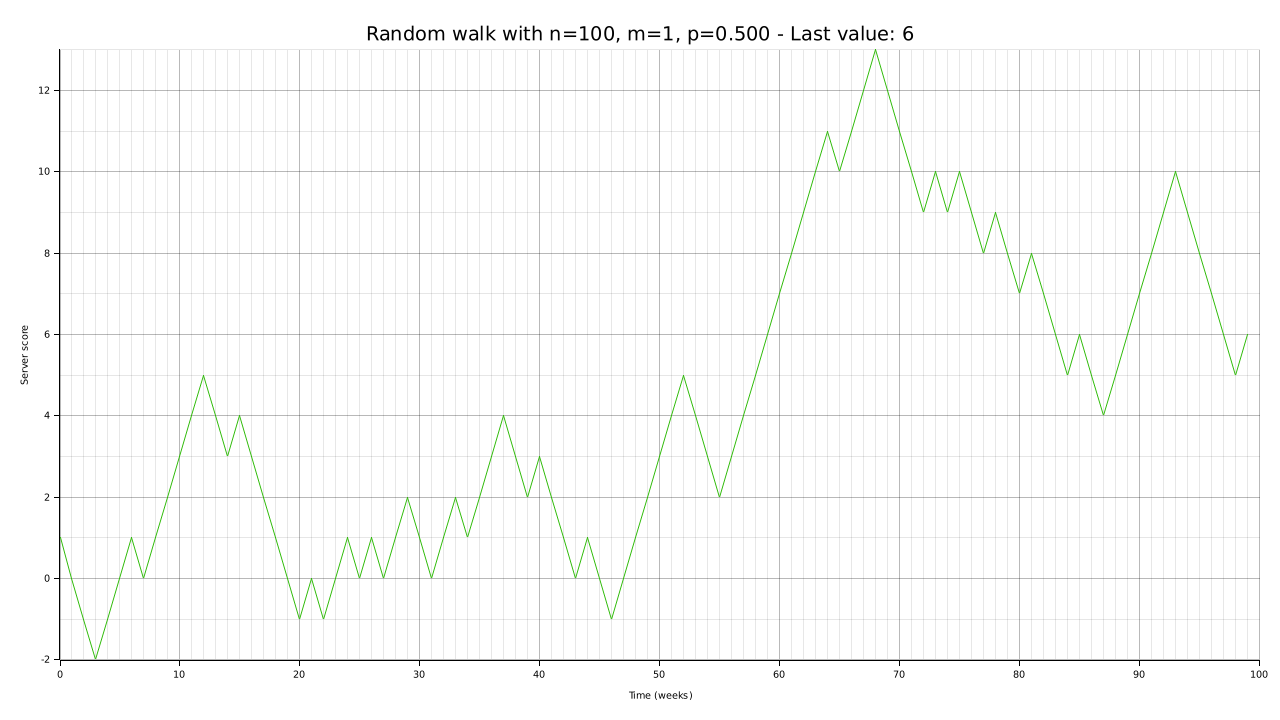
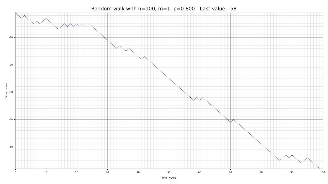
First, let’s give our CLI utility a test using low numbers and different parameters for the violation probability. We will use a single attacker for this specific test.

cargo run --bin plotter -- -W 1280 -H 720 -n 100 -p 0.2 -o output/random-walk-small-02.png
cargo run --bin plotter -- -W 1280 -H 720 -n 100 -p 0.5 -o output/random-walk-small-05.png
cargo run --bin plotter -- -W 1280 -H 720 -n 100 -p 0.8 -o output/random-walk-small-08.png

To demonstrate that with a high number of trials the random walk tends towards its expected value, let’s try again with a much higher number of weeks. Unlike in the previous articles, with a fast and memory-efficient rust implementation we can really push with the parameters:

cargo run --bin plotter -- -W 1280 -H 720 -n 1000000 -p 0.5 -o output/random-walk-big-05.png

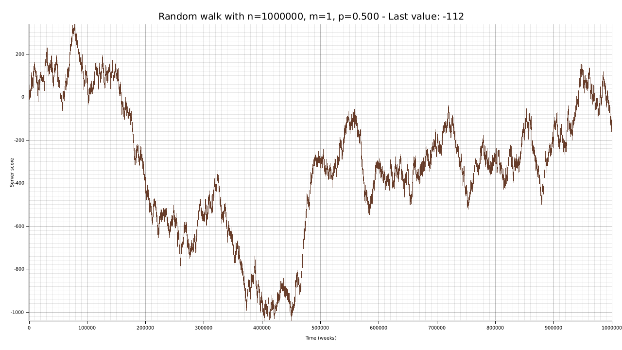
We see that with $p = 0.5$ the final value of the random walk tends to $0$, which is the expected value. We can see this further by drawing more random walks:

cargo run --bin plotter -- -W 1280 -H 720 -n 1000000 -p 0.5 -t 10 -o output/random-walk-big-05-t10.png

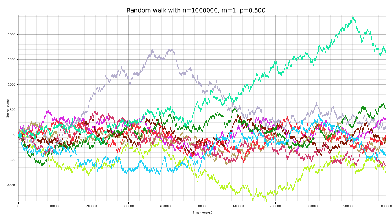
Though the random walks tend to their expected value, we see some fluctuations. However, if we start letting the $m$ parameter diverge, we can see that the generated random walks are much more stable:

cargo run --bin plotter -- -W 1280 -H 720 -n 100000 -m 100 -o output/random-walk-big-05-m100.png

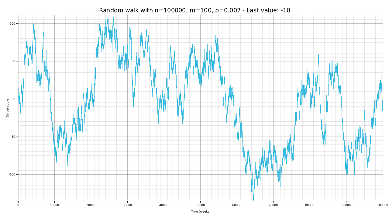
Even if visually the plot seems to be fluctuating, such fluctuations are in a $\pm 100$ range, which is quite low for $100000$ trials.

Conclusions

We built an automated simulator to generate and understand random walks. Unlike in the previous articles, our implementation is blazing-fast and memory-efficient, allowing us to really push the numbers.

We shown how, letting the $n$ and $m$ parameters diverge, the random walk’s final value tends to its expected value.