In this article we will try to understand what a Brownian motion is. First and foremost, we will discuss its definition and theoretical properties. Then, we will perform a simulation of an actual Brownian motion, approximating it in a way similar to the one used in the previous article.
The stochastic process behind the Brownian motion is known as the Wiener process. Nevertheless, the expression “Brownian motion” is often used also to describe the stochastic process itself, and not only the physical phoenomenon. We will use Brownian motion and Wiener process in an interchangeable way.
Theoretical background
The Brownian motion was discovered by the botanist Henry Brown in 1827. Richard Feynman, in one of his lectures, roughly explains how:
The Brownian movement was discovered in 1827 by Robert Brown, a botanist. While he was studying microscopic life, he noticed little particles of plant pollens jiggling around in the liquid he was looking at in the microscope, and he was wise enough to realize that these were not living, but were just little pieces of dirt moving around in the water. In fact he helped to demonstrate that this had nothing to do with life by getting from the ground an old piece of quartz in which there was some water trapped. It must have been trapped for millions and millions of years, but inside he could see the same motion. What one sees is that very tiny particles are jiggling all the time.
The Brownian motion can be intuitively defined as the motion in a fluid of a particle so small that gravity is negligible. The phoenomenon itself is not stochastic, as one could theoretically compute collision angles and trajectories of a particle with the proper tools, at least for a sufficiently small time span. However, for a relatively long period or with a relatively rough sampling, the Brownian motion can be seen as completely stochastic.
Wiener process
The Wiener process $W_t$ is the stochastic process behind the Brownian motion. It is defined by four properties:
- $\Pr(W_0 = 0) = 1$
- $W_t$ has independent increments
- $W_t$ has Gaussian increments, i.e. $W_t - W_s \sim N(0, t - s)$ for $0 \le s \lt t$
- $W_t$ is continuous in $[0, t]\ \forall t$
Random walk convergence
A Wiener process can be constructed starting with a random walk. Recalling the Homework 7, a random walk $S_n$ can be defined as follows:
Then, we can define a new stochastic process $W_n(t)$:
First, we can notice that the way $W_n$ is defined implies the following:
- $W_n(0) = 0$ always, so $\Pr(W_n(0) = 0) = 1$
- $X_i, X_j$ are independent $\forall i, j : i \ne j$, so $W_n$ has independent increments
- As $S_n$ is scaled by a factor of $\sqrt{n}$, the Gaussian increments property is satisfied
Finally, to obtain an actual Wiener process $W_t$, we can make $n$ diverge:
2-dimensional Wiener process
Let $X_i \sim \text{Rad}(p), Y_i \sim \text{Rad}(p)$. Then we can define a 2-dimensional Wiener process in a way that is very similar to the one we just used to define a 1-dimensional Wiener process:
Stochastic Differential Equations
A Stochastic Differential Equation (also known as SDE) is a differential equation inwhich at least one term is a stochastic process. The solutions of an SDE are stochastic processes.
The most simple and known form of an SDE is the following:
where:
- $W_t$ is a stochastic process
- $a(X_t, t)$ is a deterministic parameter commonly named drift, which is unrelated to $W_t$
- $b(X_t, t)$ is a deterministic parameter commonly named diffusion, indicating the diffusion of $W_t$
Wiener process as an SDE
SDEs are often use to model systems having stochastic factors. Often, the stochastic process is intended as a “disturbance” to the deterministic processes. However, SDEs can be used to model pure stochastic processes.
For example, it is possible to express a Wiener process as an SDE like so:
Euler-Maruyama method
The Euler-Maruyama method is a method to approximate the solution of a Stochastic Differential Equation.
Consider an SDE as defined in the above section. Divide a time span $[0,T]$ into $N$ equal intervals of length $\Delta t$. Then, the local solutions for the SDE can be computed incrementally with the following formula:
Simulation
Methodology and resources
As in the previous articles, the rust programming language has been used. This ensures the simulator to be fast, safe and memory-efficient.
The plotters crate has been used to generate charts with the simulation data.
The clap crate has been used to craft a handy and convenient CLI utility
The rand and rand_distr crates have been used for random number generators
and distribution interfaces. The rand_distr crate also offers a plug-and-play
Normal distribution facility that has been used for Gaussian increments in the
Wiener process simulator.
The derive_builder crate has been used to provide a very ergonomic interface
to our simulator.
Code structure
Simulations
As in the previous articles, we can model a performed simulation as a standalone rust type:
pub struct Simulation(Vec<f64>);

impl Simulation {
    pub fn final_value(&self) -> f64 {
        self.0.last().copied().unwrap_or(0.0)
    }
}

impl Deref for Simulation {
    type Target = Vec<f64>;

    fn deref(&self) -> &Self::Target {
        &self.0
    }
}

impl<'a> IntoIterator for &'a Simulation {
    type Item = &'a f64;
    type IntoIter = std::slice::Iter<'a, f64>;

    fn into_iter(self) -> Self::IntoIter {
        self.0.iter()
    }
}
This way, we can provide custom methods for the Simulation struct while still
being able to use it as an iterator of float values.
Stochastic processes
We will also model a stochastic process as a rust trait, in a similar way the
rand crate does it for distributions:
/// Memory-capable stochastic process.
/// Similar to `rand::Distribution`, offering `sample`-like capabilities with mutable self reference.
pub trait StochasticProcess<T> {
    fn next<R: Rng + ?Sized>(&mut self, rng: &mut R) -> T;
}

impl<T, D: Distribution<T>> StochasticProcess<T> for D {
    fn next<R: Rng + ?Sized>(&mut self, rng: &mut R) -> T {
        self.sample(rng)
    }
}
Notice that we provided a blanket implementation for any type that implements
rand::Distribution, so we can use distributions provided by rand and
rand_distr as instances of StochasticProcess out of the box.
Simulator
We can use the facilities in the above sections to build a generic, process-agnostic Euler-Maruyama approximator:
#[derive(Builder)]
pub struct EulerMaruyamaSimulator<S: StochasticProcess<f64>> {
    pub process: S,
    pub drift: f64,
    pub diffusion: f64,
    pub dt: f64,
    pub t: f64,
}

impl<S: StochasticProcess<f64>> EulerMaruyamaSimulator<S> {
    pub fn n(&self) -> usize {
        (self.t / self.dt).ceil() as usize
    }

    pub fn run(&mut self) -> Simulation {
        let n = (self.t / self.dt).ceil() as usize;
        let mut data: Vec<f64> = Vec::with_capacity(n);
        let mut rng = rand::rng();

        data.push(0.0);
        for i in 1..self.n() {
            let step = self.step(data[i - 1], &mut rng);
            data.push(step);
        }

        Simulation(data)
    }

    pub fn step<R: Rng + ?Sized>(&mut self, prev: f64, rng: &mut R) -> f64 {
        let w = self.process.next(rng);
        prev + self.drift + self.diffusion * w
    }
}
Our simulator can accept any stochastic process able to produce floats as output, and can use arbitrary constant float values for drift and diffusion. This behaviour may be improved further by making the simulator accept actual functions for those last two values.
Wiener process simulation
We can model a Wiener process as a rust type implementing the
StochasticProcess trait. To perform some tests, we also implemented a
Rademacher distribution facility:
/// Rademacher distribution
#[derive(Debug, Clone)]
pub struct Rademacher(Bernoulli);

/// Wiener stochastic process with Gaussian increments
#[derive(Debug, Clone)]
pub struct WienerProcess {
    pub gaussian: Normal<f64>,
    pub current: f64,
}

impl Rademacher {
    pub fn new(p: f64) -> Result<Self, BernoulliError> {
        Bernoulli::new(p).map(Rademacher)
    }
}

impl Distribution<i8> for Rademacher {
    fn sample<R: Rng + ?Sized>(&self, rng: &mut R) -> i8 {
        if self.0.sample(rng) { 1 } else { -1 }
    }
}

impl Distribution<f64> for Rademacher {
    fn sample<R: Rng + ?Sized>(&self, rng: &mut R) -> f64 {
        if self.0.sample(rng) { 1.0 } else { -1.0 }
    }
}

impl WienerProcess {
    pub fn new(dt: f64) -> Result<Self, NormalError> {
        Normal::new(0.0, dt).map(Self::from)
    }
}

impl From<Normal<f64>> for WienerProcess {
    fn from(value: Normal<f64>) -> Self {
        WienerProcess {
            gaussian: value,
            current: 0.0,
        }
    }
}

impl StochasticProcess<f64> for WienerProcess {
    fn next<R: Rng + ?Sized>(&mut self, rng: &mut R) -> f64 {
        let dw = self.gaussian.sample(rng);
        self.current = self.current + dw;
        self.current
    }
}
Notice that our version of the Wiener process uses pure Gaussian increments using a Normal distribution with standard deviation $\sqrt(\Delta t)$.
CLI tool
Finally, we can use the clap and plotters crates to craft a clean and
simple CLI tool that performs simulations and plot them to an output file:
#[derive(Parser)]
#[command(name = "brownian", about = "Brownian motion plotter")]
struct Cli {
    /// Full time period
    #[arg(short, default_value = "10.0")]
    pub t: f64,

    /// Time definition (i.e. number of trials)
    #[arg(short, default_value = "1000")]
    pub n: u32,

    /// Time delta (dt)
    #[arg(short, long)]
    pub dt: Option<f64>,

    /// Drift
    #[arg(long, default_value = "0.0")]
    pub drift: f64,

    /// Diffusion factor
    #[arg(long, default_value = "1.0")]
    pub diffusion: f64,

    /// Width of the graph in pixels
    #[arg(short = 'W', long, default_value = "1920")]
    pub width: u32,

    /// Height of the graph in pixels
    #[arg(short = 'H', long, default_value = "1080")]
    pub height: u32,

    /// Output file
    #[arg(short, long)]
    pub output: String,
}

fn main() {
    let args = Cli::parse();
    let n = args
        .dt
        .map(|dt| (args.t / dt).ceil() as usize)
        .unwrap_or(args.n as usize);
    let dt = args.dt.unwrap_or(args.t / n as f64);

    let wiener_process = WienerProcess::new(dt).unwrap();
    let mut simulator = EulerMaruyamaSimulatorBuilder::default()
        .process(wiener_process)
        .t(args.t)
        .dt(dt)
        .drift(args.drift)
        .diffusion(args.diffusion)
        .build()
        .unwrap();

    let sim = simulator.run();

    let root = BitMapBackend::new(&args.output, (args.width, args.height)).into_drawing_area();
    root.fill(&WHITE).unwrap();

    let y_min = sim
        .iter()
        .min_by(|x, y| x.partial_cmp(y).unwrap())
        .copied()
        .unwrap_or(-(n as f64));

    let y_max = sim
        .iter()
        .max_by(|x, y| x.partial_cmp(y).unwrap())
        .copied()
        .unwrap_or(n as f64);

    let caption = format!(
        "Brownian motion simulation with t={}, dt={}, a={}, b={} - Last value: {:.3}",
        args.t,
        dt,
        args.drift,
        args.diffusion,
        sim.final_value(),
    );

    let mut chart = ChartBuilder::on(&root)
        .caption(caption, ("sans-serif", 24))
        .margin(20)
        .x_label_area_size(40)
        .y_label_area_size(40)
        .build_cartesian_2d(0.0..args.t, y_min..y_max)
        .unwrap();

    chart
        .configure_mesh()
        .x_desc("t")
        .y_desc("W(t)")
        .draw()
        .unwrap();

    let data: Vec<(f64, f64)> = sim
        .into_iter()
        .enumerate()
        .map(|(i, v)| (i as f64 / n as f64 * simulator.t, *v))
        .collect();
    chart.draw_series(LineSeries::new(data, RED)).unwrap();

    root.present().unwrap();
}
We can then invoke the CLI tool to discover how it can be used:
$ cargo run --bin plotter -- --help
Brownian motion plotter

Usage: plotter [OPTIONS] --output <OUTPUT>

Options:
  -t <T>                       Full time period [default: 10.0]
  -n <N>                       Time definition (i.e. number of trials) [default: 1000]
  -d, --dt <DT>                Time delta (dt)
      --drift <DRIFT>          Drift [default: 0.0]
      --diffusion <DIFFUSION>  Diffusion factor [default: 1.0]
  -W, --width <WIDTH>          Width of the graph in pixels [default: 1920]
  -H, --height <HEIGHT>        Height of the graph in pixels [default: 1080]
  -o, --output <OUTPUT>        Output file
  -h, --help                   Print help
Running the simulation
We can use our CLI tool to perform some simulations with different parameters:
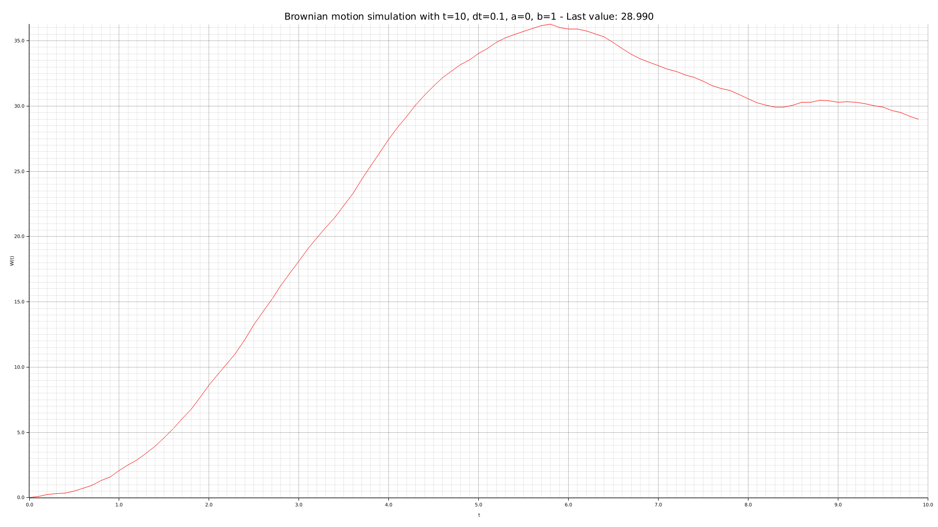
cargo run --bin plotter -- -t 10 --dt 0.1 -o output/brownian-dt01.png
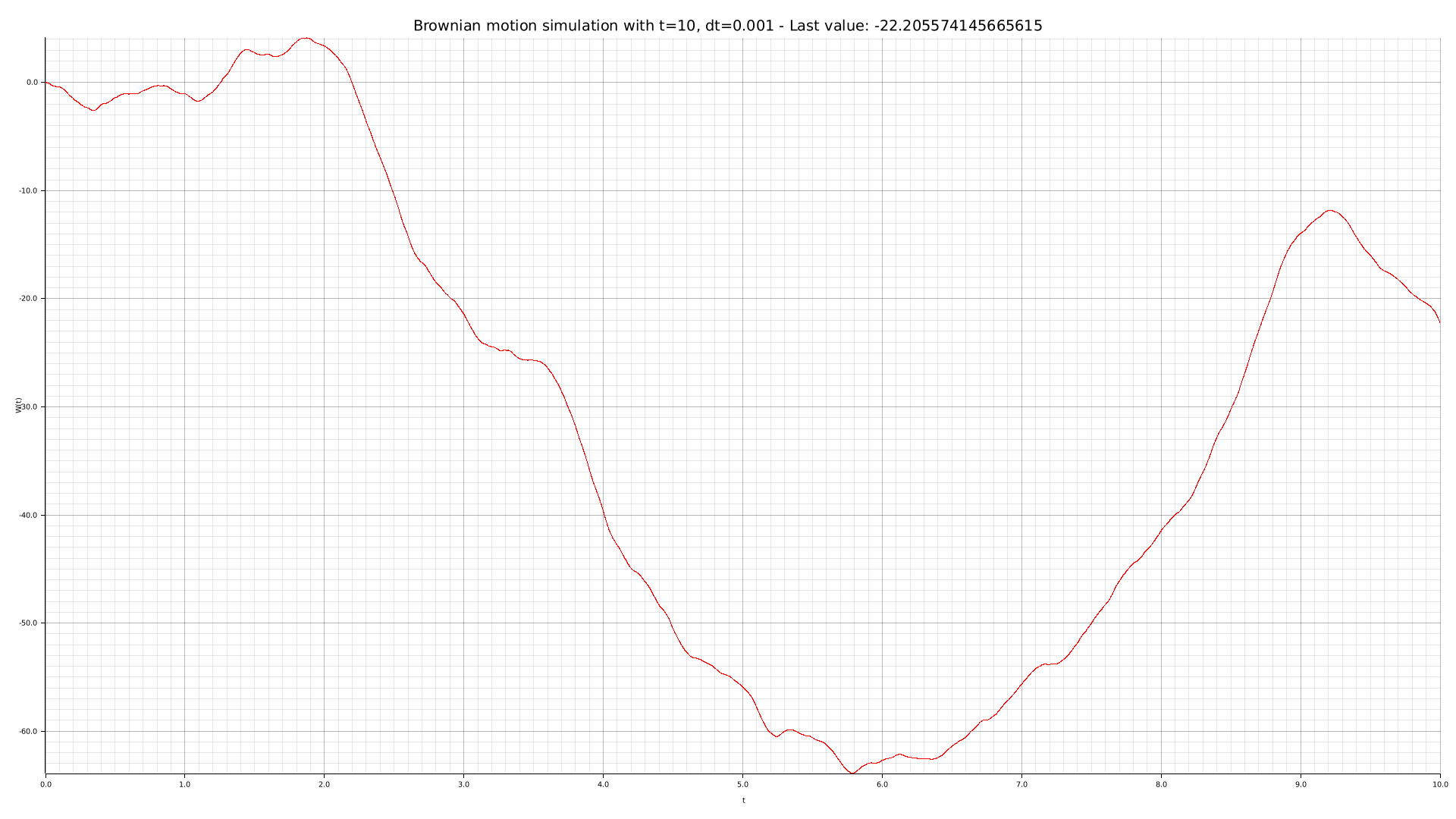
cargo run --bin plotter -- -t 10 --dt 0.001 -o output/brownian-dt0001.png
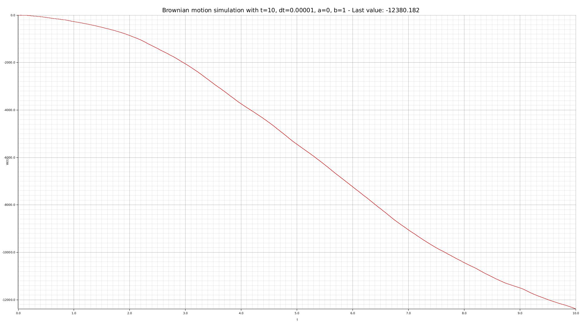
cargo run --bin plotter -- -t 10 --dt 0.00001 -o output/brownian-dt000001.png
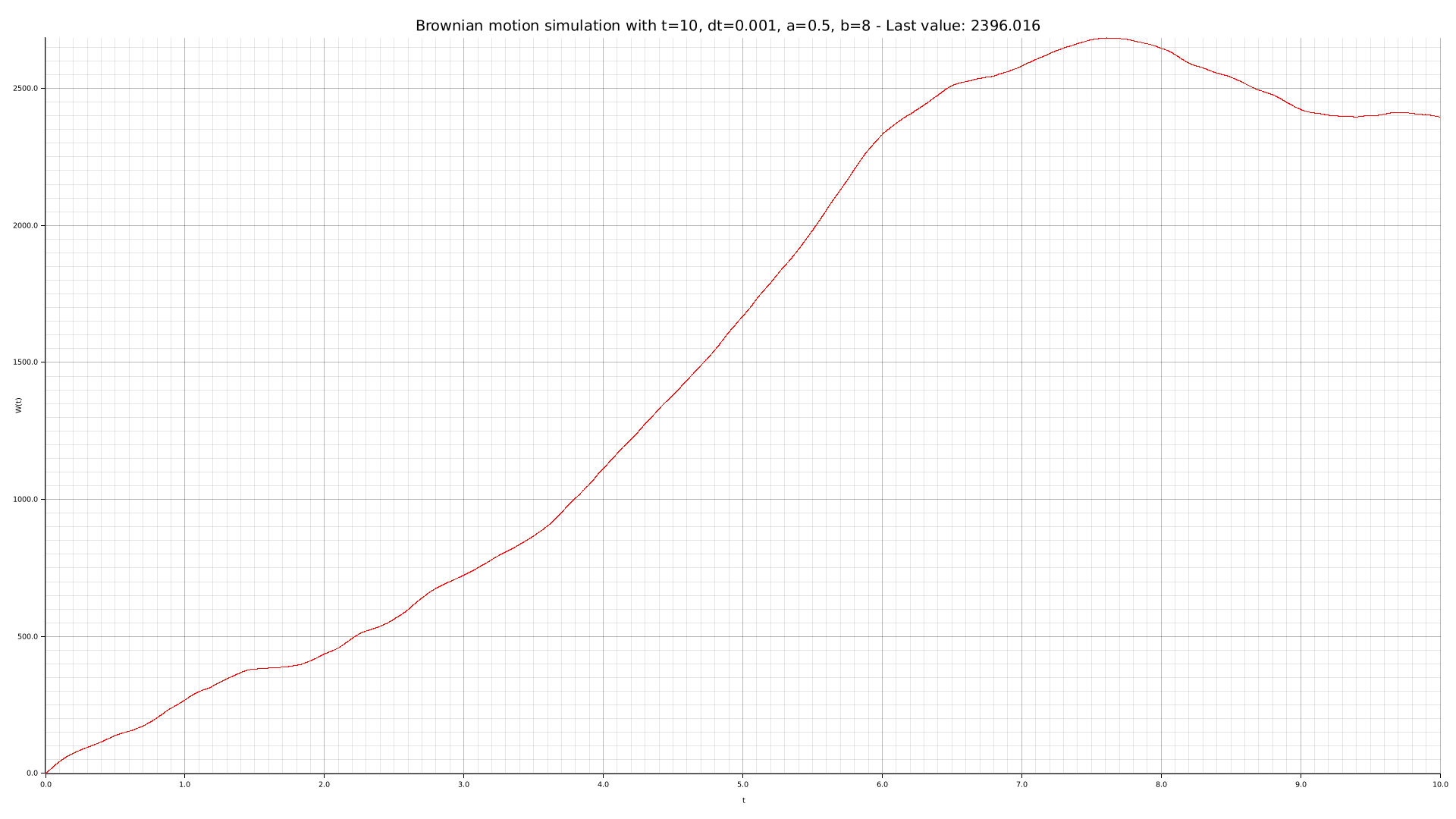
cargo run --bin plotter -- -t 10 --dt 0.001 --drift 0.5 --diffusion 8 -o output/brownian-dt0001-dr05-di8.png