In this article we will discuss the relationship between the Bernoulli processes and random walks. We will discuss the properties of both, along with their similarities and differences.

We will also take a look on the relationships between these two random processes and some important topics in statistics, such as binomial coefficients and the Tartaglia triangle.

Theoretical background

Preliminary definitions

In the previous article we gave a formal definition for the Binomial distribution and the random walk. We briefly repropose such definitions to establish a solid ground for our analysis:

Let $Y_i \sim \text{Bernoulli}(p) \ \forall \ i \in [1..n]$. We can define the Binomial random variable as follows:

$$ X \sim B(p) = \sum_{i=0}^n Y_i $$

Let $Z_i \sim \text{Rad}(p) \ \forall \ i \in [1..n]$, where $\text{Rad}(p)$ is the Rademacher distribution (which we already introduced in the previous article). We can define a random walk as follows:

$$ R \sim \text{"random walk"}(p) = \sum_{i=0}^n Z_i $$

Pascal/Tartaglia triangle

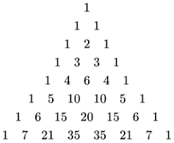
The Tartaglia (or Pascal) triangle is a visual construction that allows to easily compute binomial coefficients manually. Its construction is performed as follows:

1. Start with $1$ at the first row
2. At every lower row, each numbers is the sum of the two numbers immediately above

To map numbers in the Tartaglia triangle with a binomial coefficient $\binom{n}{k}$, consider $n$ as the row number (starting from the upper row) and $k$ as the column.

Below an example of the Tartaglia triangle is given, until $n=8$ (credits Wikimedia).

Binomial distribution and random walks

By looking at their definition, we can see that the Binomial distribution and random walks are very similar. They are both defined as the sum of a sequence of random variables.

Geometric relationship

The first important difference is that while the Bernoulli random variable is either $0$ or $1$, the Rademacher variable can be negative. Therefore, the Binomial distribution is monotonic and never decreases, while a random walk can fluctuate.

Formal relationship

The random walk and the Binomial distribution can be expressed one in the terms of the other. For example, let $R_n$ be a random walk and $S_n$ be a Binomial model.

If we think about it, they both express the very same random process, with the difference that the random walk use a signed displacement to count failures.

So we can proceed giving the following formula to derive a random walk from a Binomial process:

$$ R_n = 2 S_n - n $$

In the expression above, doubling $S_n$ and subtracting $n$ actually counts the difference between the number of successes and the number of failures, which is exactly what the random walk does.

Asymptotic analysis

Let $n \to \infty$. The Binomial distribution and the random walk tend to diffenent things.

The Binomial distribution naturally tends to a Gaussian distribution. This can be observed after rescaling and centering a Binomial variable:

$$ Z_n = \frac{S_n - np}{\sqrt{np(1 - np)}} $$

We can observe that $Z_n$ has $\mu = 0$, $\sigma^2 = 1$ and behaves as a Gaussian distribution.

On the other hand, a random walk with $n \to \infty$ tends to represent what is called a Brownian motion. A Brownian motion is used to study stochastic particle motions, and it is represented by an infinite number of random steps, just as a random walk.

Binomial coefficients and the Binomial distribution

Let $S_n \sim B(p, n)$. Let’s say we want to compute the probability of $S_n = x$. In order to achieve such condition, we must have a trajectory inwhich there are $k$ successes and $n-k$ failures. Let $\bar{X}$ be such event. Then:

$$ P(\bar{X}) = p^k (1-p)^{n-k} $$

This naturally follows from the fact that we must have $k$ successes, which occur with probability $p$ and $n-k$ failures, which occur with probability $n-p$.

Then, to count all the distinct trajectories with $k$ successes, we can use the binomial coefficient:

$$ P(S_n = k) = \binom{n}{k} p^k (1-p)^{n-k} $$

Conclusions

We analysed the relationship between the Binomial distribution and random walks.

We also introduced the Tartaglia triangle and analysed the relationship between the Binomial distribution and binomial coefficients.